The Sierpinski Triangle
Setting up the problem
We now know how to recursively apply a trisection to create complex forms that are nevertheless bounded by the initial length or perimeter of a fractal’s simplest possible order. Next we’ll leverage these and other techniques we’ve learned to develop a very interesting fractal which takes itself as the recursive element: the Sierpinski triangle.
Briefly, the Sierpinski triangle is a fractal whose initial equilateral triangle is replaced by three smaller equilateral triangles, each of the same size, that can fit inside its perimeter. You could make the argument that the middle portion of the initial triangle can accommodate a fourth triangle, but we are disallowing rotation, so that region remains empty. Further orders of the fractal replace each of the three new triangles with another three, and so forth.
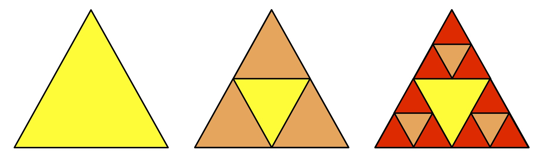
Figure 1. Sierpinski triangles, orders 0 to 2
As with the Koch curve and Koch snowflake, we first want to establish the 0th order of the fractal. In fact, it is the same as the Koch snowflake - a single equilateral triangle. Unlike the snowflake, common practice draws it with the base on the bottom, so let’s modify our code to reflect this:
import turtle

def draw(t, p):
    t.fillcolor('orange')
    t.up()
    t.goto(p[0][0], p[0][1])
    t.down()
    t.begin_fill()
    t.goto(p[1][0], p[1][1])
    t.goto(p[2][0], p[2][1])
    t.goto(p[0][0], p[0][1])
    t.end_fill()

def main():
    t = turtle.Turtle()
    t.speed()
    wn = turtle.Screen()
    wn.bgcolor("black")
    p = [[-500, -400], [0, 500], [500, -400]]
    draw(t, p)
    wn.exitonclick()

main()
I’ve also done a few things differently here, which will come in handy down the road. The first is wrapping the code that used to be in the global frame into a main() function. It’s generally good practice to write programs where everything is defined within a function. Compartmentalization helps debugging and keeps functions from accessing variables that, by virtue of being in the global frame and not residing in a specific function, you may not realize are being accessing until something breaks.
The second is in the drawing itself. This time, I’m not concerned with specifying a color for the line. Instead, by using begin_fill() and end_fill(), the line creates the shape that is filled at the moment end_fill() is called. The Sierpinski triangle is shape-based, as opposed to the line-based fractals we have created so far, so it will allow us to better see what we have drawn.
Finally, the most important innovation is our use of coordinates to guide the drawing. We use the turtle’s goto() method to tell turtle where it’s going next. The draw() function calls t.goto() four times: we first ‘pick up’ the turtle and jump to the desired coordinates, put it ‘down’ and draw our triangle with the next three goto() method calls.
To finish drawing, we end at the same coordinates we started (NB: end_fill() will fill up any space outlined between it and the begin_fill(), regardless of whether the shape is closed). Also, writing t.goto(p[0][0], p[0][1]) may seem unnecessary when we could just write t.goto(p[0]), but the importance of referencing specific index positions for coordinates will become apparent soon enough.
Loosely speaking, you could say that, for curves and snowflakes, we used a vector-based approach: the turtle’s last known position and angle provided the starting point for the next move’s direction and angle. Here we are using a raster-based approach, where everything is based on points on a grid. Both approaches have their merits, and it’s certainly possible to write code for these and other fractals using either method.
Midpoints of midpoints
Now that we have our order 0 fractal, let’s think about how we can start subdividing it. Each side of our equilateral triangle has a length of 1000, so our next order should be three triangles, each having sides of length 500. But since we’re not using vectors, we don’t have a statement like t.forward(length) that we can convert to t.forward(length // 2). A raster approach means we have to do some simple arithmetic on the list of coordinates that is p. For example, converting our original triangle to one that has the same starting vertex but only half the length looks like this:
p = [[-500, -400], [0, 500], [500, -400]]
q = [[-500, -400], [-250, 50], [0, -400]]
Our vertex stays the same (p[0] == q[0]), but the other two coordinates change. We’re now getting the midpoint between p[0] and p[1], and the midpoint between p[0] and p[2], and making those our new endpoints for q[1] and q[2]. Mathematically, the formula for computing the midpoint (x’, y’) of coordinates (x1, y1) and (x2, y2) is:
x' = (x1 + x2) / 2
y' = (y1 + y2) / 2
Using the above example,
x' = (-500 + 0)   / 2 = -250
y' = (-400 + 500) / 2 =   50
So now we know our first midpoint coordinate is (-250, 50). By the same logic, our second is (0, -400). We can abstract up a level to say that, for any pair of coordinates p1, p2, the midpoint is:
((p1[0] + p2[0]) / 2, (p1[1] + p2[1]) / 2)
We aren’t interested in explicitly defining triangles, as we were with koch(). Rather, the series of coordinates that we specify happen to make triangles. The end result may look the same, but by thinking about this in terms of coordinates and midpoints, we’ve actually vastly simplified the problem. This creates a lot of flexibility, since we just need to get the right midpoints, computed from the right vertices, and arranged in the right order.
By the same token, if we wanted the next-smaller triangle r to share the same vertex as p and q, we would apply the formula to q’s other two corners. So far, here are our three triangles:

Figure 2. Three triangles built from a common vertex
p = [[-500, -400], [0, 500],      [500, -400]]
q = [[-500, -400], [-250, 50],      [0, -400]]
r = [[-500, -400], [-375, -175], [-250, -400]]
You may be getting the sense that we will be computing midpoints quite often, so this should probably be its own function that we can call at any time, with the function’s parameters being whatever pair of coordinates whose midpoint we need to compute at any given moment:
def mid(p1, p2):
    return ((p1[0] + p2[0]) / 2, (p1[1] + p2[1]) / 2)
Making midpoints - and midpoints of midpoints - has a distinctly recursive smell to it. But before we get to the recursive case, let’s look at what it will have to address. For instance, to complete our order 1 Sierpinski triangle, we have to draw the remaining two triangles within the confines of our order 0 triangle.
To do that we’ll start A at the bottom left ((-500, -400)) to make the triangle (A, x, y). Then we’ll shift the vertex to B ((0, 500)) to make triangle (B, x, z). Finally, triangle (C, z, y) will be created from point C, at coordinates ((500, -400)). For each of these, we’ll use the mid()-generated coordinates, x, y, z. Any recursive solution will have to place us at these points. For further orders, we’ll need to place our starting vertices not just at A, B, C, but at x, y, z, and many other points.

Figure 3. Order of vertices from which midpoints are computed
Question: Can you think of a reason why choosing A, B, C as the starting vertices is preferable to choosing something like A, x, y, ie, the bottom left-hand corner of every triangle?
Determining the order of drawing
Another organizing principle for our recursive solution is that of the orders themselves. If we know that order 0 is a single triangle with sides of length n, then order 1 will have 3 triangles with sides of length n / 2, and order 2 will have 9 triangles with sides of length n / 2 / 2, etc.
So we’ll need a variable order that tells us how deep into recursion we need to go. Decrementing/incrementing order by 1 controls the depth at which we’re operating. By corollary, if main() defines order as 0 then we just go straight to the base case, which is already represented by draw() and the starting list of coordinates, p.
We learned from our Koch snowflake code that it’s a good idea to keep the recursive mechanism in a separate function from the function that draws the actual triangle, so let’s stick to that and keep draw() as it is. We’ll create a new function, sierpinski(), that will call draw() when needed. As we get into more advanced implementations of recursion, you’ll see that keeping the recursing function separate from the computing function is a common design decision.
This is what our code looks like so far:
import turtle

def draw(t, p):
    t.fillcolor('orange')
    t.up()
    t.goto(p[0][0], p[0][1])
    t.down()
    t.begin_fill()
    t.goto(p[1][0], p[1][1])
    t.goto(p[2][0], p[2][1])
    t.goto(p[0][0], p[0][1])
    t.end_fill()

def mid(p1, p2):
    return ((p1[0] + p2[0]) / 2, (p1[1] + p2[1]) / 2)

def sierpinski(t, order, p):
    draw(t, p)
    if order > 0:
        # insert recursive magic here
        # probably involving 'sierpinski(t, order - 1, p)'
        # or something like that

def main():
    t = turtle.Turtle()
    t.speed()
    wn = turtle.Screen()
    wn.bgcolor("black")

    order = 0
    p = [[-500, -400], [0, 500], [500, -400]]

    sierpinski(t, order, p)
    wn.exitonclick()

main()
This seems a bit underwhelming, since we’re not doing much more than drawing the 0 order fractal. But I want to bring attention to the structure being set up here. Looking at main(), you’ll notice that the call to draw() has been replaced by a call to sierpinski(). This makes sense, since we want to first evaluate how much recursion, if any, is needed before we start drawing, which is precisely what sierpinski() will handle. Therefore we’ll pass an additional argument order to sierpinski(), which I’ve set to 0 for the moment.
There is also something unusual going on with the base case. Most algorithms we’ve seen so far have provided usable results only upon reaching the base case - usually after we decremented some variable to 1 or 0, or met some truth condition. Sometimes we just wanted what the base case gave us (True, in the case of pal(), or a in the case of gcdRecur()). With koch() we only drew a segment when we reached the base case, because it was at the base case that we had the correctly subdivided length of line. But mostly, we were interested in the final result provided to us at the conclusion of the recusrsive cascade.
Here, we draw the 0 order fractal straight away, regardless of the value that is bound to order. This is because we want to represent the order 0 triangle first. If we didn’t, we wouldn’t have coloring for the ‘empty triangle’ in the middle. And if we waited until the end of the program, it would color over everything we’d done until that point. In fact, if we started by drawing the highest order set of triangles first, then each lower order would graphically ‘overwrite’ the previous, until we got to order 0, which would overwrite everything.
Consider what this means for the general order in which we want to draw our triangles. We can’t draw order 1 until we’ve drawn order 0, so by the same reasoning we can’t draw order 2 until we’ve drawn order 1, etc. This seems backwards from how we’ve been using recursion so far: we drew (or computed) the highest order (or n) by reaching the base case and making all the subsequent post-recursive computations. With the exception of mergeSort() we didn’t care about any of recursion’s intermediate outputs, only the final result.
If we want to draw a triangle immediately, this means we have to depart from our usual template:
def fn(n):
    if n == 1:    #or some other minimum
        return n
    else:
       return fn(n - 1) # with other computation
The need to call draw() right off the bat means it can’t sit inside an if block:
def sierpinski(t, order, p):
    draw(t, p)
    if order > 0:
        # make recursive call with sierpinski(t, order - 1, p)
If our design is valid, then each recursive call will itself trigger draw() as its first statement. Furthermore, this means that, for orders other than 0, p has to represent the right coordinates. This is where mid() comes into play.
Recall Figure 2, which showed three triangles of decreasing size built from a common vertex, p[0]. We can represent this recursively as:
def mid(p1, p2):
    return ((p1[0] + p2[0]) / 2, (p1[1] + p2[1]) / 2)

def sierpinski(t, order, p):
    draw(t, p)
    if order > 0:
        sierpinski(t, order - 1, [p[0], mid(p[0], p[1]), mid(p[0], p[2])])
In pseudocode, we might write this as follows:
- Draw the base case
- Draw the first triangle of the next order
- Keep drawing the first triangle of the next order until
order == 0
This is a good start. And you can see that we can do the same at the other two vertices of the 0 order fractal, simply by re-arranging the coordinates we want to pass to mid():

Figure 4. Computing midpoints based on p
If we translate these next two triangle calculations into code, we’ll have:
def sierpinski(t, order, p):
    draw(t, p)
    if order > 0:
        sierpinski(t, order - 1, [p[0], mid(p[0], p[1]), mid(p[0], p[2])])
        sierpinski(t, order - 1, [p[1], mid(p[0], p[1]), mid(p[1], p[2])])
        sierpinski(t, order - 1, [p[2], mid(p[2], p[1]), mid(p[0], p[2])])
Running this code for order 1 gives us the correct drawing.
At this point, you may think that we only have a partial solution: a series of triangles of decreasing size, with each series anchored at one of the three vertices of the base case triangle. In other words, there will be a lot of triangles missing. However, if you run it for, say, order == 4, you’ll see that we have created a complete solution. Why is this?
Stepping through the code
Here’s our final code for an order 2 triangle. I’ve included a bit that will be very clarifying: a list of colors that will fill each triangle based on the order we’re in at the moment.
import turtle

def draw(t, color, p):
    t.fillcolor(color)
    t.up()
    t.goto(p[0][0], p[0][1])
    t.down()
    t.begin_fill()
    t.goto(p[1][0], p[1][1])
    t.goto(p[2][0], p[2][1])
    t.goto(p[0][0], p[0][1])
    t.end_fill()

def mid(p1, p2):
    return ((p1[0] + p2[0]) / 2, (p1[1] + p2[1]) / 2)

def sierpinski(t, order, p):
    colormap = ['red', 'orange', 'yellow', 'green', 'blue', 'violet']
    draw(t, colormap[order], p)
    if order > 0:
        sierpinski(t, order-1, [p[0], mid(p[0], p[1]), mid(p[0], p[2])])
        sierpinski(t, order-1, [p[1], mid(p[0], p[1]), mid(p[1], p[2])])
        sierpinski(t, order-1, [p[2], mid(p[2], p[1]), mid(p[0], p[2])])

def main():
    t = turtle.Turtle()
    t.speed()
    wn = turtle.Screen()
    wn.bgcolor("black")
    p = [[-500, -400], [0, 500], [500, -400]]
    sierpinski(t, 2, p)
    wn.exitonclick()

main()
The recursive calls may seem a bit intimidating, but all we are doing is computing appropriate coordinates for each triangle in a given order. draw() always jumps to and draws the set of coordinates p that is correct for that moment. If you’re feeling skeptical, here is a print-traced version of the code that will show you the outputs while the drawing happens:
import turtle

call = 0

def draw(t, color, p):
    t.fillcolor(color)
    t.up()
    t.goto(p[0][0], p[0][1])
    t.down()
    t.begin_fill()
    t.goto(p[1][0], p[1][1])
    t.goto(p[2][0], p[2][1])
    t.goto(p[0][0], p[0][1])
    t.end_fill()

def mid(p1, p2):
    return ((p1[0] + p2[0]) / 2, (p1[1] + p2[1]) / 2)

def sierpinski(t, order, p):
    global call
    call += 1
    print('\ncall is', call)
    colormap = ['red', 'orange', 'yellow', 'green', 'blue', 'violet']
    print('  draw', colormap[order], 'at', p)
    draw(t, colormap[order], p)
    print('     outer call done, order =', order)
    if order > 0:
        sierpinski(t, order-1, [p[0], mid(p[0], p[1]), mid(p[0], p[2])])
        print('       1st recursive call done, order =', order)
        sierpinski(t, order-1, [p[1], mid(p[0], p[1]), mid(p[1], p[2])])
        print('       2nd recursive call done, order =', order)
        sierpinski(t, order-1, [p[2], mid(p[2], p[1]), mid(p[0], p[2])])
        print('       3rd recursive call done, order =', order)

def main():
    t = turtle.Turtle()
    t.speed()
    wn = turtle.Screen()
    wn.bgcolor("black")
    p = [[-500, -400], [0, 500], [500, -400]]
    sierpinski(t, 2, p)
    wn.exitonclick()

main()
You may want to run the print-trace program and consult the output as we step through the code. Keep in mind that this isn’t any more difficult to trace through than any other code using multiple recursive calls - all the heuristics that we established with prior algorithms still hold. The added advantage with the Sierpinski triangle is seeing it drawn in real time, so mapping the recursion to the code will be easier - plus the final result is color-coded!
A word on the recursive calls: if each triangle must fit three unique triangles within it, then we’ll clearly need three instances where sierpinski() calls itself. Of course, once we have specified three recursive calls within our function, this means that we will have three calls every time the function recurses.
As with any function with multiple recursive calls, the most important thing to remember is that the first recursive call continues recursing that first call until it reaches the ‘bottom’ or ‘leaf’, in this case when order == 0. Put another way, it is recursion executing in its usual depth-first fashion. Put a third way, this initial, depth-first run is exactly what Figure 2 represents.
In terms of our colors, we have the following:
order == 2 == 'yellow'
order == 1 == 'orange'
order == 0 == 'red'
This is the correct order of drawing, since as I pointed out above, the base case always gets drawn first. And indeed, the first triangle is yellow, with a length of 1000 for each side.
Once we’ve drawn the first triangle, we pass into the if block, since order == 2, and encounter the first recursive call:
sierpinski(t, order-1, [p[0], mid(p[0], p[1]), mid(p[0], p[2])])
This call keeps the bottom left vertex as-is (p[0]) and calls mid() twice to get the new length, 500, that is appropriate to an order 1 triangle. However, we still aren’t done with this call, as order != 0. So one more time around with the same call yields a red triangle, still with the same starting vertex, but this time with a length of 250, as p[1] and p[2] in the ‘orange order’ have once again been modified to what’s needed for the ‘red order’:
p at yellow: [[-500, -400], [0, 500], [500, -400]]
p at orange: [[-500, -400], (-250.0, 50.0), (0.0, -400.0)]
p at red:    [[-500, -400], (-375.0, -175.0), (-250.0, -400.0)]
So far we’ve replicated the original series of three triangles that we had with p, q, r in Figure 2 above, but as we saw, the code is a complete solution, so let’s keep going.
Also, keep in mind that all of these calls are opening and closing frames, based on where we are in the program execution. Seeing the call tree should make this more clear:
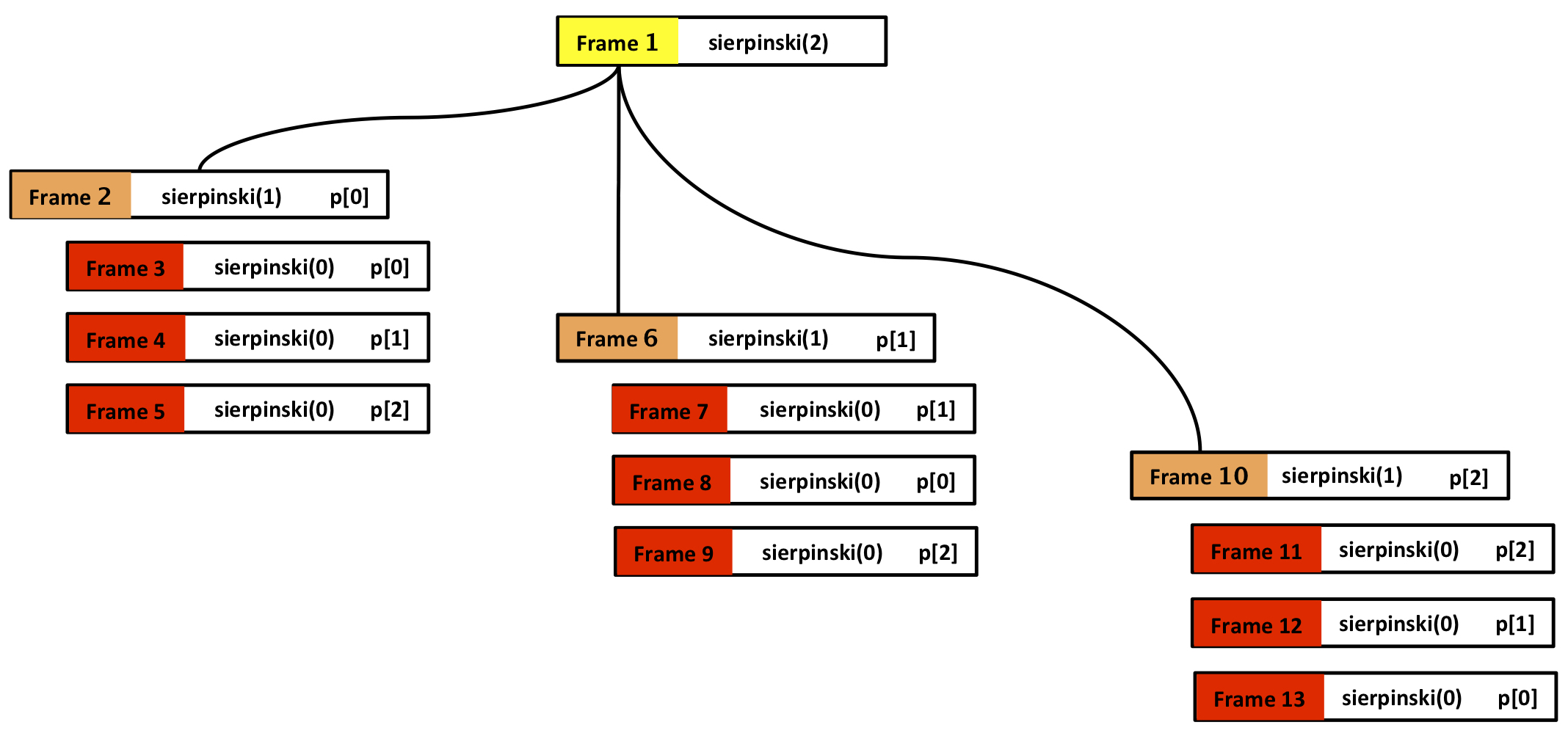
Figure 5. Call tree for an order 2 Sierpinski triangle
This further helps to discern the order of drawing. Since the recursive call whose triangle is anchored at p[0] is first, we will first see all possible triangles drawn from the perspective of p[0] at coordinates (-500, -400). This is equivalent to the first, left-most depth-first traversal of the call tree. This is represented in calls 1-3 in Figure 6.
But since frame 2 is at order == 1 we can compute the remaining two recursive calls, that is, the remaining two red triangles at order == 0, whose starting vertices are at p[1] and p[2], respectively. So now we have calls 4-5 sorted out as well.
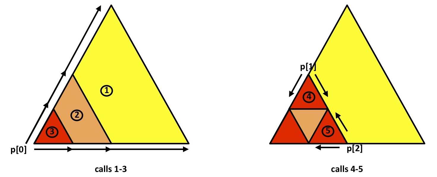
Figure 6. Calls 1-3 and 4-5
Having computed everything for frame 2, we return to frame 1, where we move on to the second recursive call, p[1], which is the vertex at the apex of the triangle. We don’t have anything to draw in frame 1 (we already did that, as we’ve now passed into the if block), so we open frame 6, draw the orange triangle and, in frame 7, the smaller red triangle, where both triangles are using p[1] == (0, 500). This takes care of calls 6-7.
For calls 8-9, we repeat the same logic as above: since frame 6 is at order == 1, we compute the remaining two red triangles, and return to frame 1 by way of frame 6:
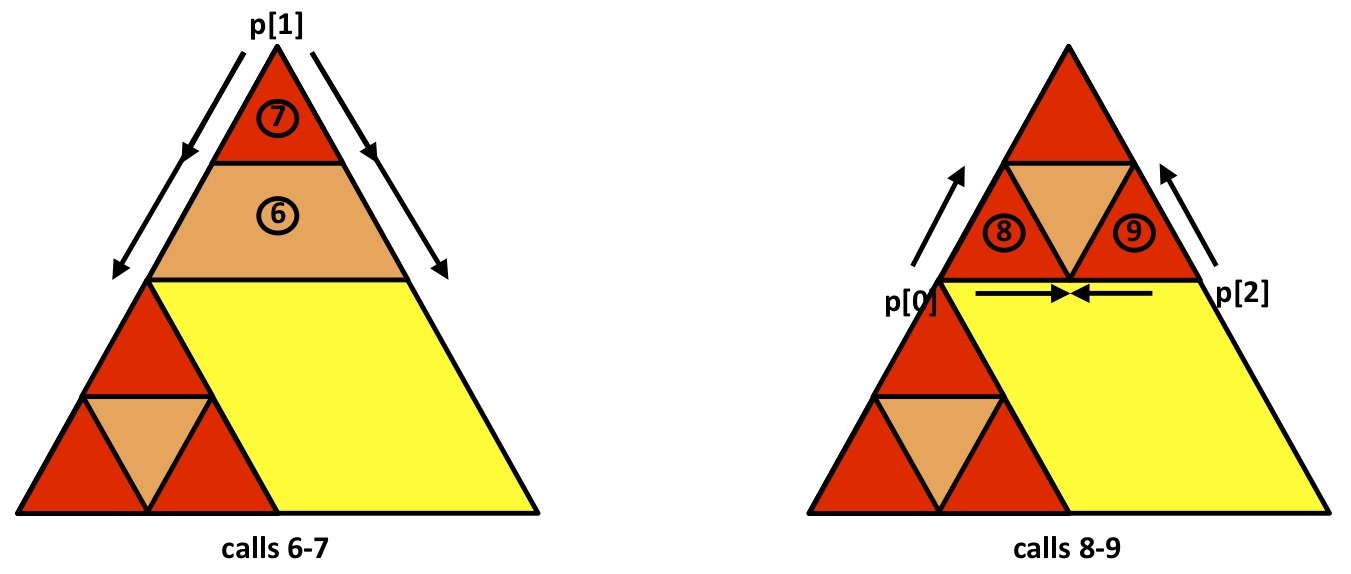
Figure 7. Calls 6-7 and 8-9
At the final recursive call p[2] in frame 1, all we have left is to fill in the bottom right of the base case triangle. By now you can see the pattern: in frames 10 and 11 p[2] is the starting vertex, providing us with calls 10-11. Finally, we add the last two red triangles, p[1] followed by p[0], for calls 12-13:
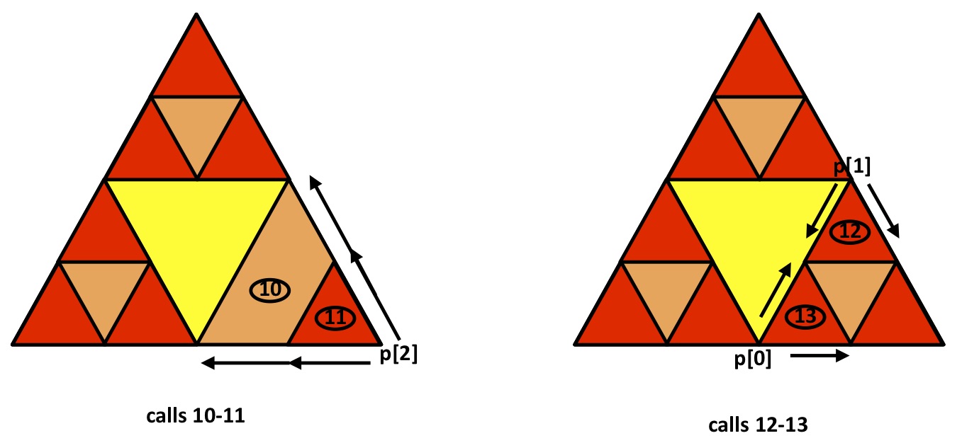
Figure 8. Calls 10-11 and 12-13
The important bit in all of this is being able to follow the order of recursive calls, which, as I’ve said, is exactly the same as any other function that uses multiple recursion. I’ve omitted some discussion about how the various coordinates get passed and re-computed, but you should take a moment to trace through how this works, as it’s very elegant.
Heuristics and Exercises
♦ In the case of the Sierpinski triangle, we wanted to ensure that lower-order drawing didn’t obscure higher-level triangles. To do this, every time sierpinski() called itself, draw() would be the first statement executed. This meant that, at the leaf level, only the base case was triggered, and the recursive calls were skipped.
♦ By keeping the recursing function separate from the computing function, you can use ongoing results of recursion as inputs for further computation. We used this technique with sierpinski() to ‘outsource’ the drawing of triangles, just as mergeSort() ‘outsourced’ its merging/sorting needs to merge().
♦ If you can write the base case and the minimally recursive case (ie, one recursion), you may well have solved the problem for any recursive depth.
Exercise: Implement a recursive solution for the Sierpinski triangle using a vector-based approach. What parts of the raster-based code can you retain?
Exercise: The Sierpinski carpet is a variation that takes a square as its base case. Each square is divided into nine equal squares, and only the central square is preserved. Write a recursive implementation for the Sierpinski carpet using a raster-based approach.
Credit: Some of this material adapted from Chapter 5.8 of Problem Solving with Algorithms and Data Structures using Python